A Compositional Framework for Scientific Model Augmentation

- Teaching computers to do science
- Model Augmentation and Synthesis
- Arbitrary models are complex, but transformations are simpler
- Project Repo github.com/jpfairbanks/SemanticModels.jl
Machine Augmentation of Scientists
- Scientists are busy writting papers
- Papers are a low bandwidth medium, because of imprecision
- We want to build AI scientists
Science as nested optimization
Fitting the data is a regression problem:
$$\ell^* = \min_{h\in {H}} \ell(h(x), y)$$
Institutional process of discovery is
$$\max_{{H}\in \mathcal{M}} expl(h^*)$$ where expl is the explanatory power of a class of models $H$.
- The explanatory power is some combination of
- generalization,
- parsimony,
- and consistency with the fundamental principles of the field.
Modeling Frameworks
Most frameworks are designed before the models are written
| Domain | ||
|---|---|---|
| Algebra |  |
|
| Learning |  |
|
| Optimization |  |
|
| Modeling |  |
SemanticModels is a post hoc modeling framework
Statistical / ML models are accurate
Fitting curves to data is good, but doesn't explain the data.
Scientific Models are Mechanistic
Mechanistic models are more explainable than black box or statistical models. They posit driving forces and natural laws that drive the evolution of systems over time.
We call these simulations when necessary to distinguish from model
- Benefits: more explainable, more generalizable
- Cons: lower Accuracy, less flexible
SIR model of disease
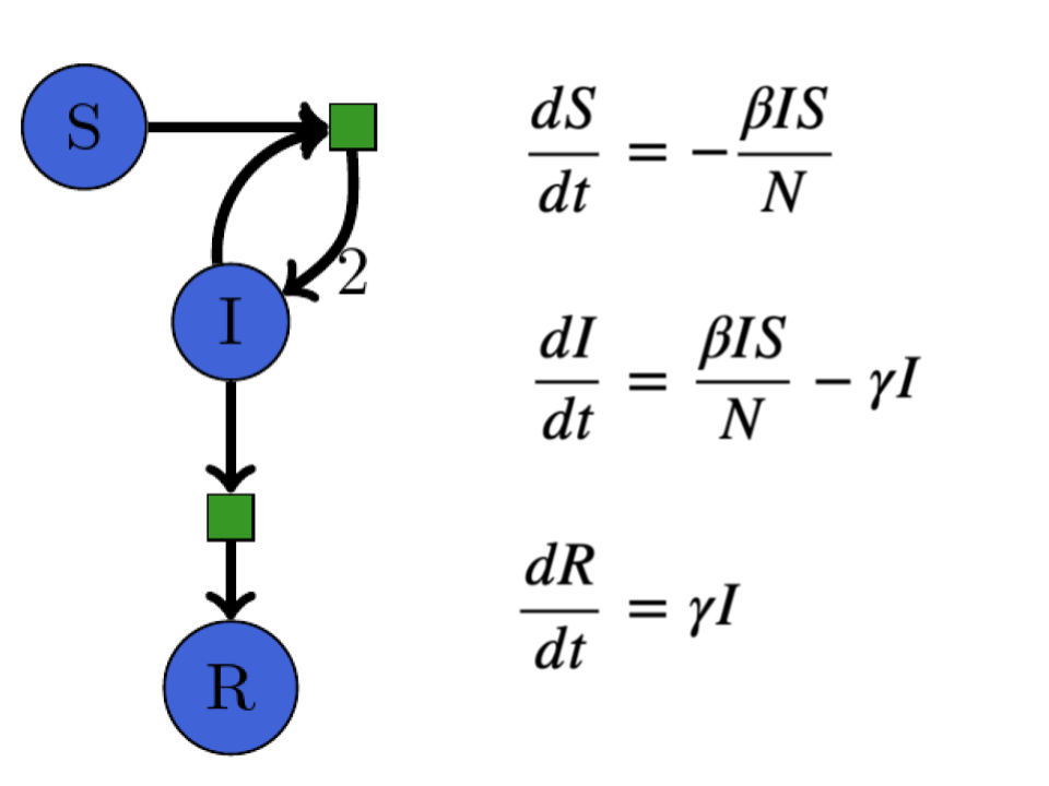 A Petri net -> ODE equivalence
Predictions
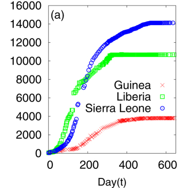 Ebola Outbreak Data
(a) Cumulative number of infected individuals as a function of time (day) for the three countries Guinea, Liberia and Sierra Leone.
A Khalequea, and P Senb, "An empirical analysis of the Ebola outbreak in West Africa" 2017
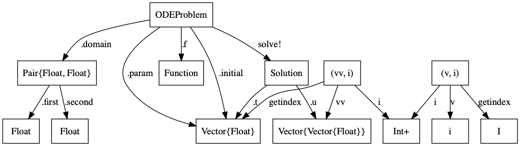
ODE Based Implementation
This is a "real world" implementation of SIR modeling in Julia taken from Epirecipes Cookbook (Simon Frost)
module SIRModel
using DifferentialEquations

function sir_ode(du, u, p, t)
    #Infected per-Capita Rate
    β = p[1]
    #Recover per-capita rate
    γ = p[2]
    #Susceptible Individuals
    S = u[1]
    #Infected Individuals
    I = u[2]
    du[1] = -β * S * I
    du[2] = β * S * I - γ * I
    du[3] = γ * I
end

#Param = (Infected Per Capita Rate, Recover Per Capita Rate)
param = [0.1,0.05]
#Initial Params = (Susceptible Individuals, Infected by Infected Individuals)
init = [0.99,0.01,0.0]
tspan = (0.0,200.0)

sir_prob = ODEProblem(sir_ode, init, tspan, param)

sir_sol = solve(sir_prob, saveat = 0.1);
Agent based simulation
""" Agent Models is a hypothetical ABM framework"""
module AgentModels

abstract type AgentModel end
mutable struct StateModel <: AgentModel
    states
    agents
    transitions
end

solve(m::StateModel) = return thesolution(m)
end
using AgentModels #<- hypothetical ABM framework

numinfected() = sum(a.==:I)
infection(x) = rand(Float64) < numinfected() ? :I : :S
recovery(x) = rand(Float64) < ρ ? :I : :R

function main(nsteps)
    n = 20
    a = fill(:S, n)
    ρ = 0.5 + randn(Float64)/4 # chance of recovery
    μ = 0.5 # chance of immunity
    T = Dict(S=>infection, I=>recovery)
    sam = StateModel([:S, :I, :R], a, T, zeros(Float64,3))
    distribution = solve!(sam, nsteps)
    return distribution
end

main(150)
Model Augmentation as a Lens
We want scientists to program using lenses
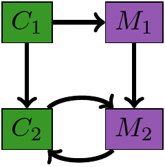 Module Augmentation as a Lens
What should the $M_1, M_2$ be?
Objects from a Category!
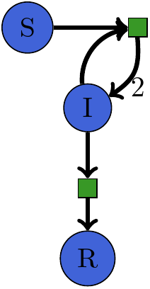 Petri Net for SIR
Petrinet SIR Model
using Petri

function main()
    @variables S, I, R
    N = +(S,I,R)

    Δ = [(S+I, 2I),
         (I, R)]

    m = Petri.Model(Δ)
    p = Petri.Problem(m, SIRState(100, 1, 0), 50)
    soln = Petri.solve(p)
    (p, soln)
end
p, soln = main()
Semantic Models Applies Category Theory
A novel modeling environment that builds and manipulates models in this category theory approach.
Contributions:
- We take general code as input
- Highly general and extensible framework
- Goal: Transformations are compositional
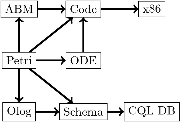
Converting Models between Categories
Models can be represented in different categories, for example, SIR as an OLOG.

Type Graphs
- The TypeGraph of a Julia Program looks a lot like the OLOG of the program it runs
- Computers are good at type checking
- Can we embed our semantics into the type system?
Functorial Semantics?
Can we make this rigorous?
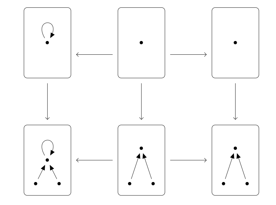
Structural Model Changes
Modifying models using a Grammar of rewrite rules.
Double Push Outs over structured cospans (Cicala Thesis, 2019)
Petrinet Model
using Petri

function main()
    @variables S, I, R
    N = +(S,I,R)

    Δ = [(S+I, 2I),
        (I, R),]

    m = Petri.Model(Δ)
    p = Petri.Problem(m, SIRState(100, 1, 0), 50)
    soln = Petri.solve(p)
    (p, soln)
end
p, soln = main()
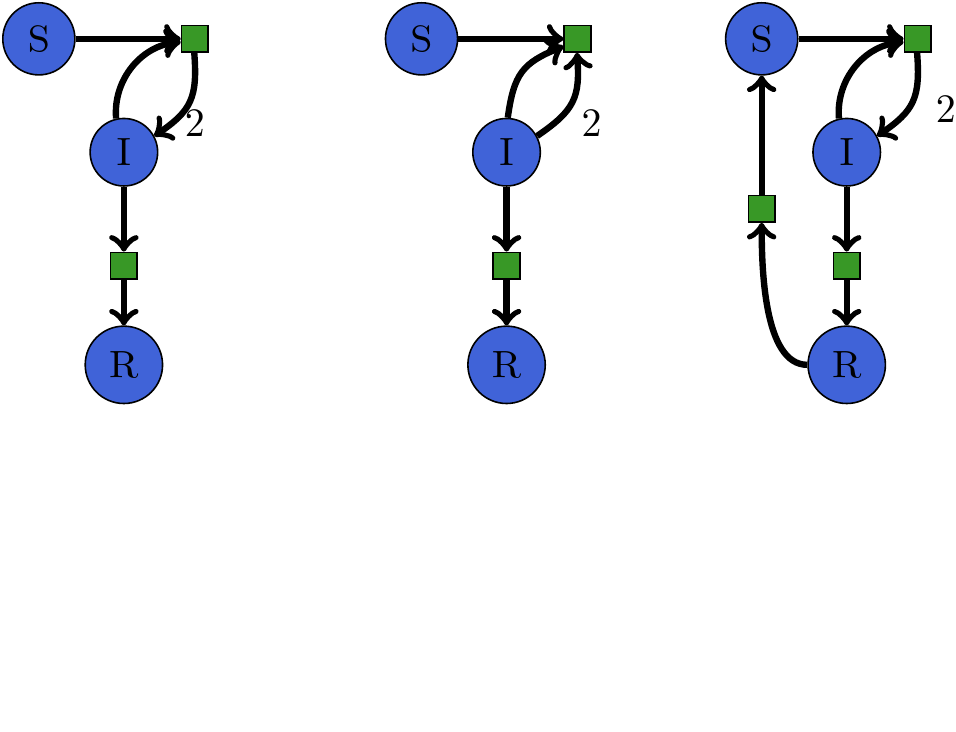
SIR -> SIRS
SIRS model as code
using Petri

function main()
    @variables S, I, R
    N = +(S,I,R)

    Δ = [(S+I, 2I),
        (I, R),
        (R, S)]

    m = Petri.Model(Δ)
    p = Petri.Problem(m, SIRState(100, 1, 0), 50)
    soln = Petri.solve(p)
    (p, soln)
end
p, soln = main()
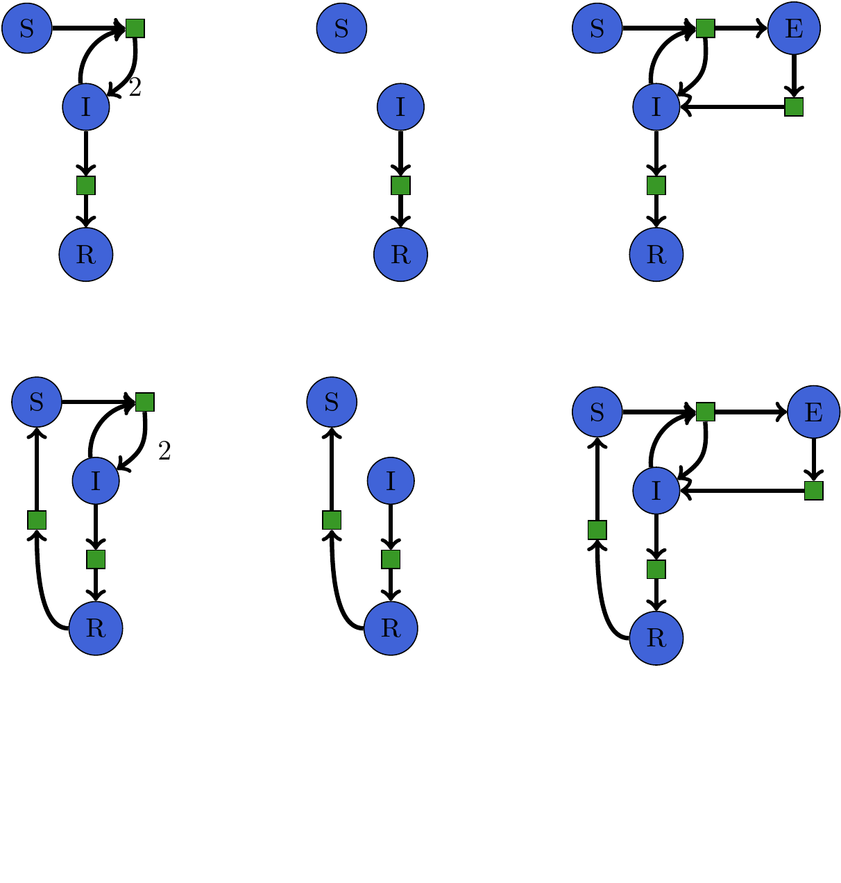
Software Interface for Rewriting Models
states = [S, I, R]

sir = Petri.Model(states,[(I, R), (S+I, 2I)])
ir = Petri.Model(states, [(I, R)])
seir = Petri.Model(states, [(I, R), (S+I, I+E), (E, I)])
rule = Span(sir, ir, seir)

# the root of the bottom of DPO
irs = Petri.Model(states, [(I, R), (R, S)])

sirs, seirs = solve(DPOProblem(rule, irs))
SEIRS Model as Declarative Code
using Petri

function SEIRSmain()
    @variables S, E, I, R
    N = +(S,E,I,R)

    Δ = [(S+I, I+E),
         (E, I),
         (I, R),
         (R, S)
    ]

    m = Petri.Model(Δ)
    p = Petri.Problem(m, SEIRState(100, 0, 1, 0), 150)
    soln = Petri.solve(p)
    (p, soln)
end
p, soln = SEIRSmain()
SEIRS Model as Imperative Code
:(##δ#754(state) = begin
          begin
              begin
                  state.I > 0 || return nothing
                  state.I -= 1
              end
              state.R += 1
          end
      end)
 :(##δ#755(state) = begin
          begin
              begin
                  state.S > 0 || return nothing
                  state.I > 0 || return nothing
                  state.S -= 1
                  state.I -= 1
              end
              begin
                  state.I += 1
                  state.E += 1
              end
          end
      end)
 :(##δ#756(state) = begin
          begin
              begin
                  state.E > 0 || return nothing
                  state.E -= 1
              end
              state.I += 1
          end
      end)
 :(##δ#757(state) = begin
          begin
              begin
                  state.R > 0 || return nothing
                  state.R -= 1
              end
              state.S += 1
          end
end)
Compiler / Disassembler
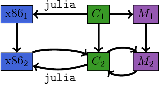 Module Augmentation as a Lens
SEIRS Model as x86 Assembly
A tiny portion of the model!
    .section    __TEXT,__text,regular,pure_instructions
; Function ##δ#788 {
; Location: rewrite.jl:127
; Function getproperty; {
; Location: rewrite.jl:148
    decl    %eax
    movl    8(%esi), %eax
;}
; Function >; {
; Location: operators.jl:286
; Function <; {
; Location: int.jl:49
    decl    %eax
    testl   %eax, %eax
;}}
    jle L37
; Function -; {
; Location: int.jl:52
    decl    %eax
    addl    $-1, %eax
;}
; Function setproperty!; {
; Location: sysimg.jl:19
    decl    %eax
    movl    %eax, 8(%esi)
;}
; Function getproperty; {
; Location: sysimg.jl:18
    decl    %eax
    movl    16(%esi), %eax
;}
; Function +; {
; Location: int.jl:53
    decl    %eax
    addl    $1, %eax
;}
; Function setproperty!; {
; Location: sysimg.jl:19
    decl    %eax
    movl    %eax, 16(%esi)
;}
    decl    %eax
    movl    %eax, (%edi)
    movb    $2, %dl
    xorl    %eax, %eax
    retl
L37:
    movb    $1, %dl
    xorl    %eax, %eax
; Location: rewrite.jl:127
    retl
    nopw    (%eax,%eax)
;}
Compiling Petri.Model to ODEProblem
f(du, state, p, t) = begin
    du.S = (-p[1] * (((state.β * state.S) * state.I)
                      / ((state.S + state.I) + state.R)))
            + p[3] * (state.μ * state.R)

    du.I = (p[1] * (((state.β * state.S) * state.I)
                      / ((state.S + state.I) + state.R)))
            + -p[2] * (state.γ * state.I)

    du.R = ((p[2] * (state.γ * state.I))
            + -p[3] * (state.μ * state.R))
end

function main()
  param = [0.1,0.05]
  init = [0.99,0.01,0.0]
  tspan = (0.0,200.0)

  prob = ODEProblem(f, init, tspan, param)

  sol = solve(prob);
end
Functorial Semantics?
Can we make this rigorous?
Conclusion
SemanticModels.jl github.com/jpfairbanks/SemanticModels.jl is a foundational technology for teaching machines to reason about scientific models
SemanticModels.jl combines DPO rewriting with Lenses for model augmentation for science!
$SemanticModels = Codification \circ Categorification \circ Science $
Open Questions
- Which scientific modeling frameworks can be categorified?
- How can we compute DPO rewriting for general categories?
- What other modeling activities have CT formalizations?
Acknowledgements